Zero-Inflated and Hurdle INAR(1) Models

Provides tools for estimating Zero-Inflated INAR(1) (ZI-INAR(1)) and Hurdle INAR(1) (H-INAR(1)) models using 'Stan'. It allows users to simulate time series data for these models, estimate parameters, and evaluate model fit using various criteria. Functions include model estimation, simulation, and likelihood-based metrics. The zero-inflated and hurdle INAR(1) methods are described by Yang et al. (2025) . Zero-inflated models also support Conway-Maxwell-Poisson innovations.

The First-order Integer-valued Autoregressive (INAR(1)) model with zero-inflated (ZI-INAR(1)) and hurdle (H-INAR(1)) innovations is widely used in studying integer-valued time-series data, such as crime count and heatwave frequency. This work implemented the INAR(1) models in Stan. The package now also supports zero-inflated INAR(1) models with Conway-Maxwell-Poisson (CMP) innovations.

Installation

You can install ZIHINAR1 from GitHub with:

remotes::install_github("fushengyy/ZIHINAR1")

Or you can install the released version of ZIHINAR1 from CRAN with:

install.packages("ZIHINAR1")

Basic Features get_stanfit()

The package contains main function named get_stanfit().

stan_fit <- get_stanfit(mod_type, distri, y, n_pred = 4,
                        thin = 2, chains = 1, iter = 2000, warmup = iter/2,
                        seed = NA, M = NULL,
                        cmp_version = c("fast", "reference"),
                        cmp_tail_tol = 1e-6, tail_action = c("warn", "error"), ...)

• mod_type: Character string indicating the model type. Use "zi" for zero-inflated models and "h" for hurdle models.

• distri: Innovation distribution. Options:

  • "poi": Poisson
  • "nb": Negative Binomial
  • "gp": Generalized Poisson (ZI only)
  • "cmp": Conway-Maxwell-Poisson (ZI only)

• y: A numeric vector of integers representing the observed data.

• n_pred: Integer specifying the number of time points for future predictions (default is 4).

• thin: Integer indicating the thinning interval for Stan sampling (default is 2).

• chains: Integer specifying the number of Markov chains to run (default is 1).

• iter: Integer specifying the total number of iterations per chain (default is 2000).

• warmup: Integer specifying the number of warmup iterations per chain (default is iter/2).

• seed: Numeric seed for reproducibility (default is NA).

• M: CMP innovation cutoff. The default is the larger of 300 and max(y).

• cmp_version: CMP Stan implementation, either "fast" (default) or "reference". Both use the same likelihood and priors.

• cmp_tail_tol: Tolerance for the CMP omitted probability mass bound (default is 1e-6).

• tail_action: Use "warn" (default) or "error" when the CMP tail bound exceeds the tolerance. Increase M and refit if this happens.

• ...: Additional arguments passed to rstan::stan().

Example

The following are examples showing how to fit the INAR(1) model when data is generated from a zero-inflated Negative Binomial (ZINB) distribution.

library(ZIHINAR1)
y_data <- data_simu(n = 100, alpha = 0.5, rho = 0.3, lambda = 5, disp = 2, 
                    mod_type = "zi", distri = "nb")
stan_fit <- get_stanfit(mod_type = "zi", distri = "nb", y = y_data, n_pred = 5, 
                        iter = 2000, chains = 1, warmup = 500, 
                        thin = 2, seed = 42)
#> 
#> SAMPLING FOR MODEL 'anon_model' NOW (CHAIN 1).
#> Chain 1: 
#> Chain 1: Gradient evaluation took 0.000174 seconds
#> Chain 1: 1000 transitions using 10 leapfrog steps per transition would take 1.74 seconds.
#> Chain 1: Adjust your expectations accordingly!
#> Chain 1: 
#> Chain 1: 
#> Chain 1: Iteration:    1 / 2000 [  0%]  (Warmup)
#> Chain 1: Iteration:  200 / 2000 [ 10%]  (Warmup)
#> Chain 1: Iteration:  400 / 2000 [ 20%]  (Warmup)
#> Chain 1: Iteration:  501 / 2000 [ 25%]  (Sampling)
#> Chain 1: Iteration:  700 / 2000 [ 35%]  (Sampling)
#> Chain 1: Iteration:  900 / 2000 [ 45%]  (Sampling)
#> Chain 1: Iteration: 1100 / 2000 [ 55%]  (Sampling)
#> Chain 1: Iteration: 1300 / 2000 [ 65%]  (Sampling)
#> Chain 1: Iteration: 1500 / 2000 [ 75%]  (Sampling)
#> Chain 1: Iteration: 1700 / 2000 [ 85%]  (Sampling)
#> Chain 1: Iteration: 1900 / 2000 [ 95%]  (Sampling)
#> Chain 1: Iteration: 2000 / 2000 [100%]  (Sampling)
#> Chain 1: 
#> Chain 1:  Elapsed Time: 0.656 seconds (Warm-up)
#> Chain 1:                1.818 seconds (Sampling)
#> Chain 1:                2.474 seconds (Total)
#> Chain 1:
get_est(distri = "nb", stan_fit = stan_fit)
#>             Mean         SD    Median       Q2.5     Q97.5      Rhat 95%_HPD_Lower 95%_HPD_Upper
#> alpha  0.4698743 0.05105897 0.4761154 0.36081446 0.5589632 0.9999792   0.361243245     0.5591202
#> rho    0.2258471 0.12798091 0.2228731 0.02060225 0.4858715 1.0024684   0.005271078     0.4496370
#> lambda 4.4128266 0.74546675 4.3652389 3.12326655 6.0788370 1.0063409   2.824085820     5.7147138
#> phi    1.5557630 0.74007545 1.3769369 0.64861912 3.4650565 1.0020000   0.500559232     2.9273579
get_mod_sel(y = y_data, mod_type = "zi", distri = "nb", stan_fit = stan_fit)
#>      EAIC     EBIC      DIC    WAIC1    WAIC2
#> 1 531.541 541.9215 526.9322 526.6891 526.9263
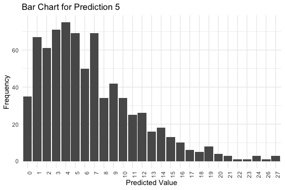
get_pred(stan_fit = stan_fit)
#> $summary
#>          Mode Median IQR Min Max
#> y_pred.1    6      7   5   1  36
#> y_pred.2    4      6   6   0  33
#> y_pred.3    3      6   6   0  43
#> y_pred.4    3      6   6   0  34
#> y_pred.5    4      5   6   0  27
#> 
#> $plots
#> $plots[[1]]

#> 
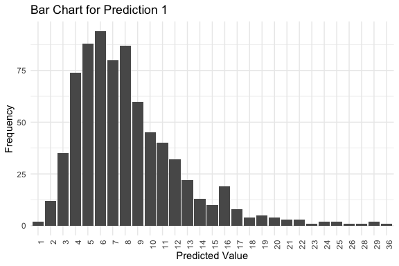
#> $plots[[2]]

#> 
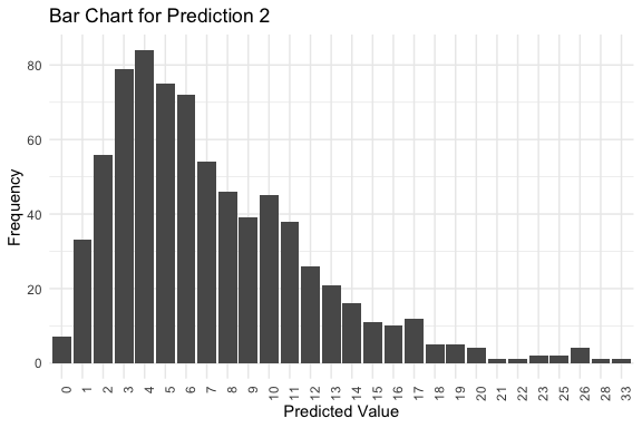
#> $plots[[3]]

#> 
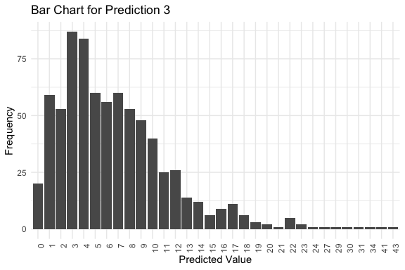
#> $plots[[4]]

#> 
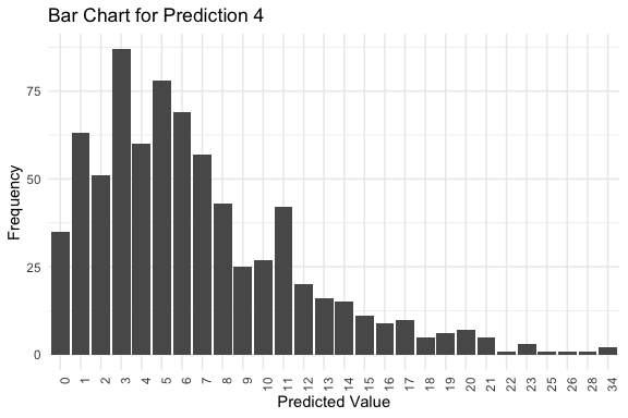
#> $plots[[5]]

Example with CMP innovations

For CMP, disp in data_simu() is the dispersion parameter nu reported by get_est(). The parameter lambda is the CMP rate.

set.seed(42)
y_cmp <- data_simu(n = 100, alpha = 0.5, rho = 0.3, lambda = 2.5, disp = 1.2,
                   mod_type = "zi", distri = "cmp")
fit_cmp <- get_stanfit(mod_type = "zi", distri = "cmp", y = y_cmp, n_pred = 5,
                       iter = 2000, chains = 4, warmup = 1000, seed = 42)
get_est(distri = "cmp", stan_fit = fit_cmp)
get_mod_sel(y = y_cmp, mod_type = "zi", distri = "cmp", stan_fit = fit_cmp)
get_pred(stan_fit = fit_cmp)