extr
Extinction Risk Estimation
Estimates extinction risk from population time series under a drifted Wiener process using MLE and observation-error-and-autocovariance-robust estimators, with confidence intervals based on the w-z method.
extr
The goal of extr is to estimate finite-horizon extinction risk from population time series under a density-independent (drifted Wiener) model, with support for both naive MLE and observation-error-and-autocovariance-robust (OEAR) variance estimation.
Installation
# CRAN release
install.packages("extr")

# GitHub version (may be newer than CRAN)
# install.packages("remotes") # if needed
remotes::install_github("hakoyamah/extr")
Main function
ext_di()
ext_di() estimates population growth rate, variance, and extinction
probability from a time series of population sizes. It supports two
variance estimators: the default naive maximum-likelihood estimator
(method = "naive") and an observation-error-and-autocovariance-robust
estimator (method = "oear"). Confidence intervals for extinction
probability are based on the $w$-$z$ method.
Example
The following example uses the Yellowstone grizzly bear time series from Dennis et al. (1991), digitized from Fig. 5. The published series is a running 3-year sum (3-year moving total).
library(extr)
dat <- data.frame(
  Time = 1959:1987,
  Population = c(
    44, 47, 46, 44, 46, 45, 46, 40, 39, 39, 42, 44, 41, 40,
    33, 36, 34, 39, 35, 34, 38, 36, 37, 41, 39, 51, 47, 57, 47
  )
)
Probability of decline to 1 individual within 100 years:
ext_di(dat, th = 100)
#> --- Estimates ---
#>                                                       Estimate
#> Probability of decline to 1 within 100 years (MLE): 9.4128e-05
#> Growth rate (MLE):                                   0.0023556
#> Environmental variance (MLE):                          0.01087
#> Unbiased variance:                                    0.011273
#> AIC for the distribution of N:                          165.06
#>                                                                        CI
#> Probability of decline to 1 within 100 years (MLE):  (1.4586e-13, 0.5653)
#> Growth rate (MLE):                                  (-0.038814, 0.043525)
#> Environmental variance (MLE):                       (0.0070464, 0.020885)
#> Unbiased variance:                                                      -
#> AIC for the distribution of N:                                          -
#>
#> --- Data Summary ---
#>                               Value
#> Current population size, nq:     47
#> xd = ln(nq / ne):            3.8501
#> Sample size, q + 1:              29
#>
#> --- Input Parameters ---
#>                                                         Parameter
#> Time unit:                                                  years
#> Extinction threshold of population size, ne:                    1
#> Time window for extinction risk evaluation (years), th:     100.0
#> Significance level, alpha:                                   0.05
Probability of decline to 10 individuals within 100 years:
ext_di(dat, th = 100, ne = 10)
#> --- Estimates ---
#>                                                       Estimate
#> Probability of decline to 10 within 100 years (MLE):  0.096852
#> Growth rate (MLE):                                   0.0023556
#> Environmental variance (MLE):                          0.01087
#> Unbiased variance:                                    0.011273
#> AIC for the distribution of N:                          165.06
#>                                                                         CI
#> Probability of decline to 10 within 100 years (MLE):  (1.0699e-05, 0.9898)
#> Growth rate (MLE):                                   (-0.038814, 0.043525)
#> Environmental variance (MLE):                        (0.0070464, 0.020885)
#> Unbiased variance:                                                       -
#> AIC for the distribution of N:                                           -
#>
#> --- Data Summary ---
#>                               Value
#> Current population size, nq:     47
#> xd = ln(nq / ne):            1.5476
#> Sample size, q + 1:              29
#>
#> --- Input Parameters ---
#>                                                         Parameter
#> Time unit:                                                  years
#> Extinction threshold of population size, ne:                   10
#> Time window for extinction risk evaluation (years), th:     100.0
#> Significance level, alpha:                                   0.05
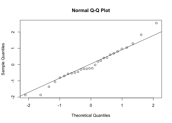
With QQ plot:
ext_di(dat, th = 100, ne = 10, qq_plot = TRUE)
#> --- Estimates ---
#>                                                       Estimate
#> Probability of decline to 10 within 100 years (MLE):  0.096852
#> Growth rate (MLE):                                   0.0023556
#> Environmental variance (MLE):                          0.01087
#> Unbiased variance:                                    0.011273
#> AIC for the distribution of N:                          165.06
#>                                                                         CI
#> Probability of decline to 10 within 100 years (MLE):  (1.0699e-05, 0.9898)
#> Growth rate (MLE):                                   (-0.038814, 0.043525)
#> Environmental variance (MLE):                        (0.0070464, 0.020885)
#> Unbiased variance:                                                       -
#> AIC for the distribution of N:                                           -
#>
#> --- Data Summary ---
#>                               Value
#> Current population size, nq:     47
#> xd = ln(nq / ne):            1.5476
#> Sample size, q + 1:              29
#>
#> --- Input Parameters ---
#>                                                         Parameter
#> Time unit:                                                  years
#> Extinction threshold of population size, ne:                   10
#> Time window for extinction risk evaluation (years), th:     100.0
#> Significance level, alpha:                                   0.05
Using the OEAR variance estimator:
ext_di(dat, th = 100, method = "oear")
#> --- Estimates ---
#>                                                                Estimate
#> Probability of decline to 1 within 100 years (OEAR plug-in): 5.1099e-10
#> Growth rate (MLE):                                            0.0023556
#> Process variance (OEAR):                                      0.0043077
#> AR(1) pre-whitening rho:                                       -0.52522
#> Bartlett lag truncation (j):                                          4
#>                                                                                  CI
#> Probability of decline to 1 within 100 years (OEAR plug-in): (1.6408e-23, 0.027088)
#> Growth rate (MLE):                                            (-0.038814, 0.043525)
#> Process variance (OEAR):                                     (0.0027924, 0.0082765)
#> AR(1) pre-whitening rho:                                                          -
#> Bartlett lag truncation (j):                                                      -
#>
#> --- Data Summary ---
#>                               Value
#> Current population size, nq:     47
#> xd = ln(nq / ne):            3.8501
#> Sample size, q + 1:              29
#>
#> --- Input Parameters ---
#>                                                         Parameter
#> Time unit:                                                  years
#> Extinction threshold of population size, ne:                    1
#> Time window for extinction risk evaluation (years), th:     100.0
#> Significance level, alpha:                                   0.05
Irregularly spaced observations
The default ML method can use irregularly spaced observations directly. Under the drifted Wiener process model, the likelihood is evaluated for the observed time intervals, so no interpolation is needed.
dat_irregular <- subset(
  dat,
  Time %in% c(1959, 1960, 1962, 1965, 1969, 1974, 1980, 1987)
)

ext_di(dat_irregular, th = 100, ne = 10)
A mostly complete annual series with a few missing observations can also
be supplied using NA values.
dat_with_na <- data.frame(
  Time = 1959:1975,
  Population = c(
    44, 47, NA, 44, 46, 45, 46, NA, 39, 39,
    42, 44, NA, 40, 33, 36, 34
  )
)

ext_di(dat_with_na, th = 100, ne = 10)
For the OEAR method, mild missingness can be treated as a pragmatic
effective-diffusion approximation. Avoid using method = "oear" when
missing observations are numerous or observation intervals are highly
heterogeneous.
ext_di(dat_with_na, th = 100, ne = 10, method = "oear")