Geometric Methods for Nonparametric Regression and Density Estimation

Provides geometric methods for nonparametric regression and density estimation on data represented as coordinate matrices or weighted graphs. Methods include local polynomial smoothing, model-averaged local polynomial smoothing, local polynomial lifting trend filtering, synchronized local polynomial lifting trend filtering, order-2 Gaussian and logistic trend filtering, graph low-pass filtering, and Hessian-energy regression. Methodological references include Gajer and Ravel (2025) "Adaptive Geometric Regression for High-Dimensional Structured Data" , Fan and Gijbels (1996, ISBN:9780412983214), Wang et al. (2016) "Trend Filtering on Graphs" < https://www.jmlr.org/papers/v17/15-147.html>, and Kim et al. (2009) "Semi-Supervised Regression Using Hessian Energy" < https://papers.nips.cc/paper/3741-semi-supervised-regression-using-hessian-energy-with-an-application-to-semi-supervised-dimensionality-reduction>.

geosmooth

geosmooth provides geometric methods for nonparametric regression and density estimation on data represented as coordinate matrices or weighted graphs. It includes local polynomial smoothing, model-averaged local polynomial smoothing, local polynomial lifting trend filtering, synchronized local polynomial lifting trend filtering, one-dimensional logistic trend filtering, graph low-pass filtering, and Hessian-energy regression.

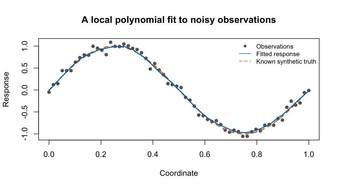
The points are observations, the solid line is a selected local polynomial fit, and the dashed line is known synthetic truth. The first-fit guide shows the code, selected settings, and how to interpret the tuning score.

For a task-based catalog of every exported function, prediction capabilities, and examples, read Finding your way around geosmooth. In an installed package, use vignette("function-guide", package = "geosmooth") or start with help("geosmooth-package", package = "geosmooth").

Browse the reference by task, functions A–Z, or synthetic datasets guide. See NEWS for migration details.

Installation

For the version currently on CRAN:

install.packages("geosmooth")
help("geosmooth-package", package = "geosmooth")

The 0.2.0 release candidate includes the guides below and requires R >= 4.1.0 and dgraphs >= 0.4.0. Its optional GRIP and edge-KK embeddings require grip >= 0.3.0. These dependency releases must be available before the candidate can complete CRAN-only validation. A source installation needs an R compilation toolchain.

Once those dependencies are published on CRAN, install the candidate with:

install.packages("pak")
pak::pkg_install("pgajer/geosmooth")
vignette("function-guide", package = "geosmooth")

The package-check and website workflows now resolve dependencies from CRAN. Their next builds and the final CRAN dependency check remain pending until dgraphs >= 0.4.0 and grip >= 0.3.0 are published. Earlier successful checks used development dependencies and do not establish CRAN-only release readiness. See the submission draft for the recorded status and remaining validation.

Quick Start

library(geosmooth)

set.seed(1)
x <- seq(0, 1, length.out = 60)
X <- cbind(x = x)
y <- sin(2 * pi * x) + rnorm(length(x), sd = 0.08)
foldid <- rep(1:5, length.out = length(y))

lps.fit <- fit.lps(
    X = X,
    y = y,
    foldid = foldid,
    support.grid = c(8L, 12L, 16L),
    degree.grid = 0:1,
    kernel.grid = "gaussian"
)

head(predict(lps.fit))

fit.lps() is the canonical local polynomial smoother (LPS) entry point. It selects support size, local polynomial degree, and kernel by cross-validation.

Method Map

Choose by the structure of your data and the penalty you need:

• LPS: local polynomial smoother, fit.lps(). Use this as the direct local-regression baseline. It predicts by fitting a local polynomial around each evaluation point.

• MALPS: model-averaged local polynomial smoother, fit.malps(). Use this when you want many local polynomial fits around observed anchors and an averaged prediction surface.

• LPL-TF: local polynomial lifting trend filtering, fit.lpl.tf() and lpl.tf.operator(). Use this when the local polynomial residual operator should be regularized by an L1 (absolute-value) trend-filtering penalty.

• SLPLiFT / S-LPL-TF: synchronized local polynomial lifting trend filtering, fit.slpl.tf() and slpl.tf.operator(). Use this when you want LPL-TF plus a quadratic synchronization penalty across overlapping local predictions.

• Graph low-pass: fit.metric.graph.lowpass() smooths a response on an undirected graph with positive edge lengths or supplied nonnegative conductances. The graph workflow explains vertex alignment, length-to-conductance conversion, and basis reuse. The observed-data heat guide covers missing responses, numerical cross-checks, and unresolved tuning choices.

• One-dimensional Gaussian trend filtering: fit.gaussian.trend.filtering() fits continuous outcomes with an order-2 piecewise-quadratic curve. assess.gaussian.trend.filtering() retunes on each outcome permutation, compares held-out MSE/MAE with a training-only mean, and reports absolute deviation and total variation. The permutation null requires exchangeability; constant mean alone under arbitrary heteroskedasticity is insufficient.

• One-dimensional logistic trend filtering: fit.logistic.trend.filtering() fits a binary outcome over a continuous predictor. The assessment function tests constancy by permutation and measures predictive improvement. Likelihood remains the default test; absolute-deviation and total-variation summaries have optional permutation tests with Holm adjustment. The logistic trend-filtering guide illustrates fitting and assessment on synthetic and Pima data.

• SSRHE: SSRHE-style Hessian-energy smoothing, fit.ssrhe.hessian.regression() and fit.ssrhe.hessian.l1.regression(). Use this as a Hessian-energy comparator with fixed-k, supplied, or graph-derived adaptive-radius neighborhoods.

Basic Examples

LPS

lps.fit <- fit.lps(
    X = X,
    y = y,
    foldid = foldid,
    support.grid = c(8L, 12L),
    degree.grid = 0:1,
    kernel.grid = "gaussian"
)

lps.pred <- predict(lps.fit, X)

MALPS

malps.fit <- fit.malps(
    X = X,
    y = y,
    degree = 1L,
    support.type = "knn",
    support.size = 12L,
    kernel = "tricube",
    support.selection = "fixed",
    coordinate.method = "coordinates"
)

LPL-TF and SLPLiFT Operators

lpl.op <- lpl.tf.operator(
    X = X,
    degree = 1L,
    support.type = "knn",
    support.size = 12L,
    kernel = "gaussian",
    coordinate.method = "coordinates"
)

slpl.op <- slpl.tf.operator(
    X = X,
    degree = 1L,
    support.type = "knn",
    support.size = 12L,
    kernel = "gaussian",
    coordinate.method = "coordinates"
)

Fitting LPL-TF and SLPLiFT currently uses the optional genlasso dependency.

if (requireNamespace("genlasso", quietly = TRUE)) {
    lpl.fit <- fit.lpl.tf(
        y = y,
        operator = lpl.op,
        lambda = 0.1,
        lambda.selection = "fixed"
    )

    slpl.fit <- fit.slpl.tf(
        y = y,
        operator = slpl.op,
        lambda1 = 0.1,
        lambda2 = 0.01,
        lambda.selection = "fixed"
    )
}

SSRHE Hessian-Energy Regression

grid <- expand.grid(x = seq(0, 1, length.out = 5),
                    y = seq(0, 1, length.out = 5))
X2 <- as.matrix(grid)
y2 <- sin(2 * pi * X2[, 1]) + 0.25 * X2[, 2]

ssrhe.fit <- fit.ssrhe.hessian.regression(
    X = X2,
    y = y2,
    k = 12L,
    tangent.dim = 2L,
    lambda1 = 0.05,
    return.local.diagnostics = FALSE
)

# Select penalties with the same fitter (use "gcv" for fully observed data).
ssrhe.cv <- fit.ssrhe.hessian.regression(
    X = X2,
    y = y2,
    k = 12L,
    tangent.dim = 2L,
    lambda.selection = "cv",
    lambda1.grid = c(0.01, 0.05, 0.2),
    cv.control = list(cv.folds = 5L)
)

The same runnable code is available in inst/examples/geosmooth_quickstart.R.

Graph Dependency Boundary

geosmooth owns smoother APIs and package-local coordinate/fixed-k paths. Graph construction and shortest-path operations are supplied by dgraphs.

That means:

• Coordinate LPS, coordinate MALPS, coordinate LPL-TF/SLPLiFT, fixed-k SSRHE, and supplied-neighborhood SSRHE are package-local geosmooth paths.
• Graph-dependent paths, including graph-geodesic MALPS/LPL-TF/SLPLiFT supports and SSRHE adaptive-radius neighborhoods, use compatible dgraphs graph objects.
• geosmooth does not currently export graph construction functions such as rKNN graph builders.

Native support currently includes:

• C++ coordinate backend for LPS CV and prediction
• C++ shared local-PCA chart backend
• C++ SSRHE Hessian-energy operator backend

Native Backends

The package includes compiled backends for LPS cross-validation and prediction, shared local-PCA chart construction, metric-graph low-pass filtering, and SSRHE Hessian-energy operators.

Validation

Focused validation:

make test
make check-fast