Soil Organic Carbon Turnover Modelling with 'C-TOOL'

Provides an 'R' interface to the 'C-TOOL' soil carbon turnover model for simulating soil organic carbon dynamics in agricultural systems. The package supports the definition of carbon inputs, management schedules, soil parameters, and temperature forcing, and includes tools for scenario analysis and calibration of selected model parameters against observed soil organic carbon stocks. The 'C-TOOL' model and related modelling framework are described by Petersen et al. (2002) , Petersen et al. (2005) , Petersen et al. (2013) , and Taghizadeh-Toosi et al. (2014) . Further applications and developments are described by Taghizadeh-Toosi et al. (2016) , Keel et al. (2017) , Taghizadeh-Toosi et al. (2020) , and Taghizadeh-Toosi and Christensen (2021) .

rCTOOL

rCTOOL is an open-source R package for running C-TOOL simulations of soil organic carbon dynamics in agricultural systems. It provides a user-friendly R interface for defining carbon inputs, management schedules, soil parameters, temperature forcing, scenario simulations, and parameter calibration.

The package builds on the C-TOOL model framework (Petersen, Olesen, and Heidmann 2002; Taghizadeh-Toosi et al. 2014) and aims to make C-TOOL-based simulations easier to configure, reproduce, document, and extend.

Installation

Once available on CRAN, rCTOOL can be installed with:

install.packages("rCTOOL")

The development version can be installed from GitHub:

# install.packages("devtools")
devtools::install_github("francagiannini/rCTOOL")

Basic example

This is a simple example of the potential use of rCTOOL. The example corresponds to one of the treatments presented by (Jensen et al. 2021) and (Jensen et al. 2022) containing the C inputs for the treatment of the spring barley crop with 4 DM Mg/ha straw incorporated into the soil at a long-term experimental station Askov, Denmark.

library(rCTOOL)
library(ggplot2)

# load data ----
data('basic_example')
data('scenario_temperature')

The basic_example dataset contains annual carbon inputs and monthly management allocation information.

head(basic_example, 2)
#>   mon  yrs id year Cin_top Cin_sub Cin_man manure_monthly_allocation
#> 1   1 1951  1 1951   3.566    0.39       0                         0
#> 2   2 1951  1 1952   3.566    0.39       0                         0
#>   plant_monthly_allocation
#> 1                        0
#> 2                        0

The scenario_temperature dataset contains monthly temperature data.

head(scenario_temperature, 2)
#>   month   yr     Tavg
#> 1     1 1951 0.890000
#> 2     2 1951 1.170714

A standard rCTOOL simulation requires five main inputs:

1. simulation period;
2. carbon inputs;
3. management configuration;
4. soil configuration;
5. temperature configuration.

# define timeperiod 
period <- define_timeperiod(
  yr_start = 1951,
  yr_end = 2019
  )

# get annual Carbon inputs 
cin <- define_Cinputs(
  management_filepath = basic_example
  )

# get management 
management <- management_config(
  management_filepath = basic_example,
  grain_monthly_allocation = rep(0, 12),
  grass_monthly_allocation = rep(0, 12),
  f_man_humification = 0.192
)

# get soil configuration 
soil <- soil_config(Csoil_init = 105, 
                   f_hum_top =  0.533,
                   f_rom_top =  0.405,
                   f_hum_sub =  0.387,
                   f_rom_sub =  0.610,
                   Cproptop = 0.55,
                   clay_top = 0.11,
                   clay_sub = 0.20,
                   phi = 0.035,
                   f_co2 = 0.628,
                   f_romi = 0.012,
                   k_fom  = 0.12,
                   k_hum = 0.0028,
                   k_rom = 3.85e-5,
                   ftr = 0.0025
                   )

Initial soil pools are calculated before running the simulation. They depend on the initial soil carbon stock, the initial C:N ratio, and the distribution of carbon among FOM, HUM, and ROM pools.

# initialize soil pools
soil_pools <- initialize_soil_pools(
  cn = 12,
  soil_config = soil
)

soil_pools <- c(soil_pools[[1]], soil_pools[[2]])

The monthly simulation is then run with run_ctool(). The verbose argument can be used to run additional diagnostic checks during the simulation.

# run rCTOOL
output <- run_ctool(
  time_config = period,
  cin_config = cin,
  m_config = management,
  t_config = scenario_temperature,
  s_config = soil,
  soil_pools = soil_pools,
  verbose = FALSE
)

The resulting output contains monthly carbon pools, soil carbon stocks, transport fluxes, and CO2 emissions.

head(output)
#>   mon  yrs  FOM_top FOM_top_decomposition substrate_FOM_decomp_top
#> 1   1 1951 3.435048            -0.1454518                0.1454518
#> 2   2 1951 3.195740            -0.2393079                0.2393079
#> 3   3 1951 2.915547            -0.2801936                0.2801936
#> 4   4 1951 2.668412            -0.5324143                0.5324143
#> 5   5 1951 2.416203            -0.6801291                0.6801291
#> 6   6 1951 2.267384            -0.7193794                0.7193794
#>   FOM_humified_top em_CO2_FOM_top       FOM_tr   FOM_sub FOM_sub_decomposition
#> 1       0.02782131      0.1172668 0.0003636294 0.1375258          -0.004587808
#> 2       0.04577366      0.1929360 0.0005982698 0.1307436          -0.007380504
#> 3       0.05359408      0.2258990 0.0007004840 0.1223929          -0.009051156
#> 4       0.10183764      0.4292456 0.0013310358 0.1324329          -0.022491038
#> 5       0.13009180      0.5483369 0.0017003226 0.1425719          -0.038361325
#> 6       0.13759943      0.5799816 0.0017984486 0.1540850          -0.052685398
#>   substrate_FOM_decomp_sub FOM_humified_sub em_CO2_FOM_sub  HUM_top
#> 1              0.004587808     0.0009878393    0.003599969 25.95689
#> 2              0.007380504     0.0015891579    0.005791346 25.96039
#> 3              0.009051156     0.0019488800    0.007102276 25.96077
#> 4              0.022491038     0.0048427332    0.017648305 25.96145
#> 5              0.038361325     0.0082598971    0.030101428 25.95782
#> 6              0.052685398     0.0113441328    0.041341265 25.94876
#>   HUM_top_decomposition substrate_HUM_decomp_top HUM_romified_top
#> 1           -0.02462729               0.02462729     0.0002955275
#> 2           -0.04226870               0.04226870     0.0005072243
#> 3           -0.05321946               0.05321946     0.0006386335
#> 4           -0.10115380               0.10115380     0.0012138456
#> 5           -0.13372738               0.13372738     0.0016047285
#> 6           -0.14665546               0.14665546     0.0017598655
#>   em_CO2_HUM_top      HUM_tr  HUM_sub HUM_sub_decomposition
#> 1     0.01546594 0.008865824 15.42058           -0.01162135
#> 2     0.02654474 0.015216730 15.42507           -0.01924719
#> 3     0.03342182 0.019159005 15.43030           -0.02481767
#> 4     0.06352458 0.036415367 15.43801           -0.05240850
#> 5     0.08398079 0.048141856 15.44536           -0.07665266
#> 6     0.09209963 0.052795966 15.45048           -0.09220968
#>   substrate_HUM_decomp_sub HUM_romified_sub em_CO2_HUM_sub  ROM_top
#> 1               0.01162135     0.0001394562    0.007298207 28.21587
#> 2               0.01924719     0.0002309662    0.012087233 28.21598
#> 3               0.02481767     0.0002978120    0.015585495 28.21612
#> 4               0.05240850     0.0006289019    0.032912535 28.21638
#> 5               0.07665266     0.0009198319    0.048137870 28.21673
#> 6               0.09220968     0.0011065161    0.057907677 28.21712
#>   ROM_top_decomposition substrate_ROM_decomp_top em_CO2_ROM_top       ROM_tr
#> 1         -0.0003677493             0.0003677493   0.0002309465 9.193731e-07
#> 2         -0.0006306740             0.0006306740   0.0003960633 1.576685e-06
#> 3         -0.0007937270             0.0007937270   0.0004984605 1.984317e-06
#> 4         -0.0015058543             0.0015058543   0.0009456765 3.764636e-06
#> 5         -0.0019886082             0.0019886082   0.0012488460 4.971521e-06
#> 6         -0.0021805722             0.0021805722   0.0013693994 5.451431e-06
#>    ROM_sub ROM_sub_decomposition substrate_ROM_decomp_sub em_CO2_ROM_sub
#> 1 31.69002         -0.0003282270             0.0003282270   0.0002061265
#> 2 31.68991         -0.0005432775             0.0005432775   0.0003411783
#> 3 31.68977         -0.0007001122             0.0007001122   0.0004396704
#> 4 31.68947         -0.0014760401             0.0014760401   0.0009269532
#> 5 31.68904         -0.0021556707             0.0021556707   0.0013537612
#> 6 31.68853         -0.0025906327             0.0025906327   0.0016269173
#>   C_topsoil C_subsoil SOC_stock C_transport em_CO2_top em_CO2_sub em_CO2_total
#> 1  57.60781  47.24813  104.8559 0.009230373  0.1329637 0.01110430    0.1440680
#> 2  57.37211  47.24572  104.6178 0.015816577  0.2198768 0.01821976    0.2380965
#> 3  57.09243  47.24246  104.3349 0.019861474  0.2598193 0.02312744    0.2829468
#> 4  56.84625  47.25992  104.1062 0.037750168  0.4937159 0.05148779    0.5452037
#> 5  56.59075  47.27697  103.8677 0.049847151  0.6335666 0.07959306    0.7131596
#> 6  56.43326  47.29310  103.7264 0.054599866  0.6734506 0.10087586    0.7743265

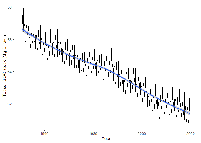
The topsoil SOC trajectory can be visualized as follows.

output$time <- as.Date(
  paste(output$yrs, output$mon, "01", sep = "-")
)

ggplot(output, aes(x = time, y = C_topsoil)) +
  geom_line() +
  geom_smooth() +
  theme_classic() +
  labs(
    x = "Year",
    y = "Topsoil SOC stock (Mg C ha-1)"
  )

## Output variables

The rCTOOL output includes time, carbon stocks, pool sizes, transport fluxes, and CO2 emissions.

Time variables:

• mon: month of the year (1-12);
• yrs: year of the simulation.

Soil carbon stocks and profile-level fluxes (Mg/ha):

• C_topsoil: carbon stock in the topsoil (0-25 cm).
• C_subsoil: carbon stock in the subsoil (26-100 cm).
• SOC_stock: total Soil Organic Carbon stock in the soil (0-100 cm).
• C_transport: carbon transported to the subsoil.
• em_CO2_top: total CO2 emissions from the topsoil.
• em_CO2_sub: total CO2 emissions from the subsoil.
• em_CO2_total: total CO2 emissions from the soil.

Fresh Organic Matter (FOM) pool:

• FOM_top: FOM in the topsoil.
• FOM_top_decomposition: monthly decomposition of FOM in the topsoil.
• substrate_FOM_decomp_top: substrate for FOM decomposition in the topsoil.
• FOM_humified_top: FOM that has been “humified” in the topsoil (becomes part of topsoil HUM).
• em_CO2_FOM_top: CO2 emissions from the decomposition of FOM in the topsoil.
• FOM_tr: FOM transported from the topsoil to the subsoil.
• FOM_sub: FOM in the subsoil.
• FOM_sub_decomposition: decomposition of FOM in the subsoil.
• substrate_FOM_decomp_sub: substrate for FOM decomposition in the subsoil.
• FOM_humified_sub: FOM that has been “humified” in the subsoil (becomes part of subsoil HUM).
• em_CO2_FOM_sub: CO2 emissions from the decomposition of FOM in the subsoil.

Humified Organic Matter (HUM) pool:

• HUM_top: HUM in the topsoil.
• HUM_top_decomposition: Decomposition of HUM in the topsoil.
• substrate_HUM_decomp_top: Substrate for HUM decomposition in the topsoil.
• HUM_romified_top: HUM that has been “romified” in the topsoil (becomes part of topsoil ROM).
• em_CO2_HUM_top: CO2 emissions from the decomposition of HUM in the topsoil.
• HUM_tr: HUM transported from the topsoil to the subsoil.
• HUM_sub: HUM in the subsoil.
• HUM_sub_decomposition: Decomposition of HUM in the subsoil.
• substrate_HUM_decomp_sub: Substrate for HUM decomposition in the subsoil.
• HUM_romified_sub: HUM that has been “romified” in the subsoil (becomes part of subsoil ROM).
• em_CO2_HUM_sub: CO2 emissions from the decomposition of HUM in the subsoil.

Resistant Organic Matter (ROM) pool:

• ROM_top: ROM in the topsoil.
• ROM_top_decomposition: Decomposition of ROM in the topsoil.
• substrate_ROM_decomp_top: Substrate for ROM decomposition in the topsoil.
• em_CO2_ROM_top: CO2 emissions from the decomposition of ROM in the topsoil.
• ROM_tr: ROM transported from the topsoil to the subsoil.
• ROM_sub: ROM in the subsoil.
• ROM_sub_decomposition: Decomposition of ROM in the subsoil.
• substrate_ROM_decomp_sub: Substrate for ROM decomposition in the subsoil.
• em_CO2_ROM_sub: CO2 emissions from the decomposition of ROM in the subsoil.

Parameter calibration

rCTOOL includes a calibration module for evaluating and calibrating selected CTOOL parameters against observed SOC stocks.

The current calibration module tests combinations of:

• f_hum_top: fraction of decomposed topsoil FOM entering the HUM pool;
• k_hum: decomposition rate of the HUM pool.

For each tested value of f_hum_top, the corresponding f_rom_top is calculated internally as:

f_rom_top = 1 - f_hum_top - f_fom_top

The only additional data required for calibration is a two-column data frame containing observed SOC stocks by year. In this example, we create a small artificial observed dataset from the simulated output only to demonstrate the workflow.

observed <- aggregate(
  C_topsoil ~ yrs,
  data = output,
  FUN = mean
)

observed <- data.frame(
  Year = observed$yrs + 1,
  SOC_obs = observed$C_topsoil
)

observed <- observed[observed$Year %in% c(1955, 1965, 1975, 1985, 1995), ]

observed
#>    Year  SOC_obs
#> 4  1955 56.10409
#> 14 1965 55.52216
#> 24 1975 54.62216
#> 34 1985 54.16431
#> 44 1995 53.38794

The tested parameter ranges are defined using min, max, and by.

calib <- ctool_calibrate(
  time_config = period,
  cinput_config = cin,
  temperature_config = scenario_temperature,
  management_config = management,
  soil_config = soil,
  observed = observed,
  f_hum_top = c(min = 0.20, max = 0.60, by = 0.10),
  k_hum = c(min = 0.0020, max = 0.0040, by = 0.0010),
  verbose = FALSE
)

summary(calib)
#> C-TOOL calibration summary
#> =========================
#> 
#> Calibration data:
#>   Observations: 5
#>   Tested combinations: 15
#> 
#> Calibrated parameters:
#>   f_hum_top
#>   k_hum
#> 
#> Parameter ranges:
#>   f_hum_top: 0.2 to 0.6 by 0.1
#>   k_hum: 0.002 to 0.004 by 0.001
#> 
#> Calibration settings:
#>   f_fom_top: 0.003
#>   cn_init: 10
#>   Ranking metric: d_index
#>   Minimize metric: FALSE
#> 
#> Best tested calibration:
#>  f_hum_top k_hum f_rom_top   d_index     RMSE        R2      Bias       MAE n
#>        0.4 0.004     0.597 0.8678099 1.038007 0.9781859 0.4954844 0.7633362 5
#> 
#> Current parameters versus best tested calibration:
#>                       Type   d_index     RMSE        R2       Bias       MAE n
#>  Current C-TOOL parameters 0.5768270 2.460624 0.9908253 -2.2206482 2.2206482 5
#>    Best tested calibration 0.8678099 1.038007 0.9781859  0.4954844 0.7633362 5
#>  f_hum_top  k_hum f_rom_top
#>      0.533 0.0028     0.405
#>      0.400 0.0040     0.597
#> 
#> Recommended parameter set:
#>                   Source f_hum_top k_hum f_rom_top   d_index     RMSE        R2
#>  Best tested calibration       0.4 0.004     0.597 0.8678099 1.038007 0.9781859
#>       Bias       MAE n
#>  0.4954844 0.7633362 5
#> 
#> Recommendation:
#>   Use the best tested calibration because it improved the selected performance metric compared with the current C-TOOL parameters.

The calibration output includes:

• the current CTOOL parameter performance;
• the best tested calibration;
• a recommended parameter set;
• full metrics for all tested parameter combinations.

Model performance is evaluated using RMSE, MAE, mean bias, R2, and the Willmott index of agreement, reported as d_index (Willmott 1981).

calib$recommended_params
#>                    Source f_hum_top k_hum f_rom_top   d_index     RMSE
#> 1 Best tested calibration       0.4 0.004     0.597 0.8678099 1.038007
#>          R2      Bias       MAE n
#> 1 0.9781859 0.4954844 0.7633362 5

If the current CTOOL parameters perform as well as or better than the tested calibration grid, ctool_calibrate() recommends keeping the current parameter set.

Comparing multiple scenarios

rCTOOL can also be used to compare multiple management or land-use scenarios. The following example uses the scenario dataset.

data('scenario')
data('scenario_temperature')

The scenario dataset contains different C input assumptions for different management s options.

• For the football court scenario we assume a well-maintained stomped ryegrass cover,

• for the organic dairy farming we assume a crop rotation with grass, maize and cereals for happy milking cows,

• and finally for the pet cemetery we assume a less healthily reygrass and a certain number of beloved dogs and cats from Viborg municipality burred in the subsoil.

Now we will play with rCTOOL to explore the implications in terms of soil C dynamics.

First lets take a look on the C inputs distribution:

period <- define_timeperiod(
  yr_start = 1951,
  yr_end = 2019
)

management <- management_config(
  manure_monthly_allocation = c(0, 0, 1, 0, 0, 0, 0, 0, 0, 0, 0, 0),
  plant_monthly_allocation = c(0, 0, 0, 8, 12, 16, 64, 0, 0, 0, 0, 0) / 100,
  grain_monthly_allocation = rep(0, 12),
  grass_monthly_allocation = rep(0, 12),
  f_man_humification = 0
)

soil <- soil_config(
  Csoil_init = 100,
  f_hum_top = 0.4803,
  f_rom_top = 0.4881,
  f_hum_sub = 0.3123,
  f_rom_sub = 0.6847,
  Cproptop = 0.47,
  clay_top = 0.1,
  clay_sub = 0.15,
  phi = 0.035,
  f_co2 = 0.628,
  f_romi = 0.012,
  k_fom = 0.12,
  k_hum = 0.0028,
  k_rom = 3.85e-5,
  ftr = 0.003
)

soil_pools <- initialize_soil_pools(
  cn = 10,
  soil_config = soil
)

Then define carbon inputs and run the model for each scenario.

treatment <- unique(scenario$treatment)

cin_treatment <- lapply(treatment, function(x) {
  define_Cinputs(
    management_filepath = subset(scenario, treatment == x)
  )
})

names(cin_treatment) <- treatment

output_treatment <- lapply(treatment, function(x) {
  out <- run_ctool(
    time_config = period,
    cin_config = cin_treatment[[x]],
    m_config = management,
    t_config = scenario_temperature,
    s_config = soil,
    soil_pools = soil_pools,
    verbose = FALSE
  )

  out$treatment <- x
  out
})

output_treatment <- data.table::rbindlist(output_treatment)

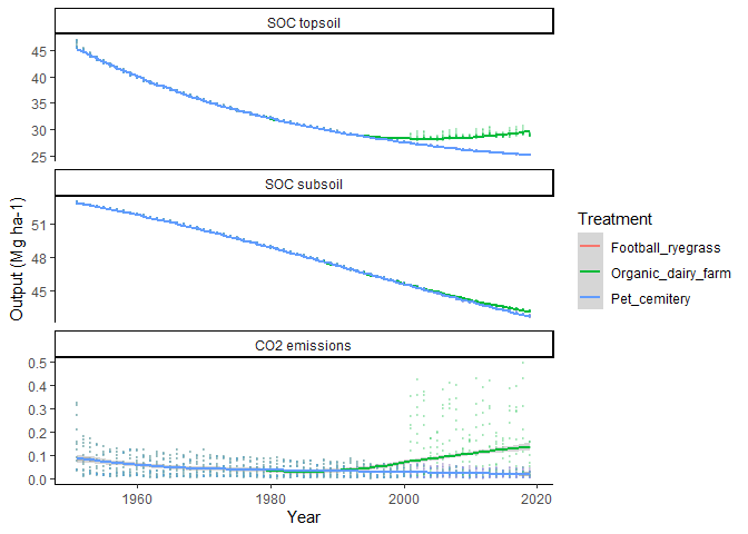
The simulated trajectories can then be compared across scenarios.

plot_df <- output_treatment[
  ,
  c("mon", "yrs", "C_topsoil", "C_subsoil", "em_CO2_total", "treatment")
]

plot_df <- reshape2::melt(
  plot_df,
  id.vars = c("mon", "yrs", "treatment")
)

labels <- c(
  C_topsoil = "SOC topsoil",
  C_subsoil = "SOC subsoil",
  em_CO2_total = "CO2 emissions"
)

ggplot(plot_df, aes(x = yrs, y = value, colour = treatment)) +
  geom_point(size = 0.02, alpha = 0.2) +
  geom_smooth() +
  facet_wrap(
    variable ~ .,
    scales = "free_y",
    ncol = 1,
    labeller = as_labeller(labels)
  ) +
  labs(
    x = "Year",
    y = "Output (Mg ha-1)",
    colour = "Treatment"
  ) +
  theme_classic()

References

Jensen, Johannes L., Jørgen Eriksen, Ingrid K. Thomsen, Lars J. Munkholm, and Bent T. Christensen. 2022. “Cereal Straw Incorporation and Ryegrass Cover Crops: The Path to Equilibrium in Soil Carbon Storage Is Short.” Journal Article. European Journal of Soil Science 73 (1). https://doi.org/10.1111/ejss.13173.
Jensen, Johannes L., Ingrid K. Thomsen, Jørgen Eriksen, and Bent T. Christensen. 2021. “Spring Barley Grown for Decades with Straw Incorporation and Cover Crops: Effects on Crop Yields and n Uptake.” Journal Article. Field Crops Research 270. https://doi.org/10.1016/j.fcr.2021.108228.
Petersen, Bjørn M., Jørgen E. Olesen, and Tove Heidmann. 2002. “A Flexible Tool for Simulation of Soil Carbon Turnover.” Journal Article. www.elsevier.com/locate/ecolmodel.
Taghizadeh-Toosi, Arezoo, Bent T. Christensen, Nicholas J. Hutchings, Jonas Vejlin, Thomas Kätterer, Margaret Glendining, and Jørgen E. Olesen. 2014. “C-TOOL: A Simple Model for Simulating Whole-Profile Carbon Storage in Temperate Agricultural Soils.” Journal Article. Ecological Modelling 292: 11–25. https://doi.org/https://doi.org/10.1016/j.ecolmodel.2014.08.016.
Willmott, Cort J. 1981. “On the Validation of Models.” Physical Geography 2 (2): 184–94.