rpsurv
Fast Royston-Parmar Flexible Parametric Survival Models
Fits Royston-Parmar flexible parametric survival models
(Royston and Parmar, 2002)
rpsurv


rpsurv fits the Royston and Parmar (2002) family of flexible
parametric survival models: the baseline distribution is a restricted
cubic spline in log time on a chosen transformed scale (proportional
hazards, proportional odds, or probit), which gives a smooth, fully
parametric, extrapolable fit without committing to a Weibull,
log-normal, or other single distribution. Covariate effects can vary
over time (tve) and be non-linear in the covariate itself (nle),
each with its own spline.
The log-likelihood and its analytic gradient are evaluated in C++ via
RcppParallel, so fitting stays fast at large sample sizes (see the
Benchmark section below). Output mirrors coxph():
print()/summary() separate interpretable covariate effects from the
baseline spline nuisance parameters, and there are
predict()/plot()/residual-diagnostic methods.
All results below are real output from the bundled brcancer data (686
rows, 299 events).
Installation
# CRAN release:
install.packages("rpsurv")

# development version:
# install.packages("remotes")
remotes::install_github("ielbadisy/rpsurv")
Fitting a model
library(rpsurv)
library(survival)

data(brcancer)
brcancer$hormon <- as.numeric(brcancer$hormon)

fit <- rpsurv(Surv(rectime, censrec) ~ hormon, data = brcancer, df = 4, scale = "hazard")
fit
#> Royston-Parmar flexible parametric survival model
#> Call:
#> rpsurv(formula = Surv(rectime, censrec) ~ hormon, data = brcancer,
#>     df = 4, scale = "hazard")
#>
#> Scale: hazard   Baseline df: 4
#> n = 686, number of events = 299
#> Log-likelihood = -2606.47, AIC = 5224.94

summary(fit)
#> Royston-Parmar flexible parametric survival model
#> Call:
#> rpsurv(formula = Surv(rectime, censrec) ~ hormon, data = brcancer,
#>     df = 4, scale = "hazard")
#>
#> Covariate effects (hazard scale):
#>           coef exp(coef) [HR] se(coef)      z Pr(>|z|)
#> hormon -0.3641         0.6949   0.1249 -2.914  0.00356 **
#> ---
#> Signif. codes:  0 '***' 0.001 '**' 0.01 '*' 0.05 '.' 0.1 ' ' 1
#>
#> Baseline spline terms:
#>                 coef se(coef)      z Pr(>|z|)
#> (Intercept) -19.5955   3.2573 -6.016 1.79e-09
#> s(logt)1      2.9925   0.5965  5.016 5.27e-07
#> s(logt)2     -0.4431   0.5711 -0.776   0.4378
#> s(logt)3      1.3573   0.8187  1.658   0.0974
#> s(logt)4     -0.8842   0.4176 -2.118   0.0342
#>
#> n = 686, number of events = 299, parameters = 6
#> Log-likelihood = -2606.47, AIC = 5224.94, BIC = 5247.15
The summary keeps the interpretable covariate hazard ratio (hormon)
separate from the baseline spline coefficients, which describe the shape
of the baseline hazard and are not individually interpretable, matching
rstpm2/flexsurv convention.
Prediction and plotting
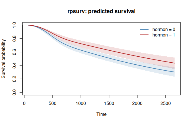
predict(fit, newdata = data.frame(hormon = c(0, 1)), times = c(500, 1000, 2000), type = "survival")
#>   id time       est
#> 1  1  500 0.8287000
#> 2  1 1000 0.6284929
#> 3  1 2000 0.4078290
#> 4  2  500 0.8776032
#> 5  2 1000 0.7241834
#> 6  2 2000 0.5362160

plot(fit, newdata = data.frame(hormon = c(0, 1)),
     col = c("steelblue", "firebrick"), main = "rpsurv: predicted survival")
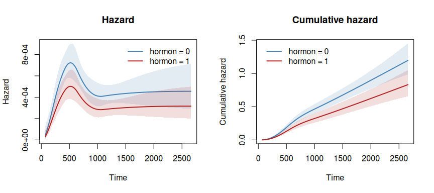
plot() draws the same profiles on the hazard and cumulative hazard
scales, each with its 95% confidence band:
op <- par(mfrow = c(1, 2))
plot(fit, newdata = data.frame(hormon = c(0, 1)), type = "hazard",
     col = c("steelblue", "firebrick"), main = "Hazard")
plot(fit, newdata = data.frame(hormon = c(0, 1)), type = "cumhaz",
     col = c("steelblue", "firebrick"), main = "Cumulative hazard")
par(op)
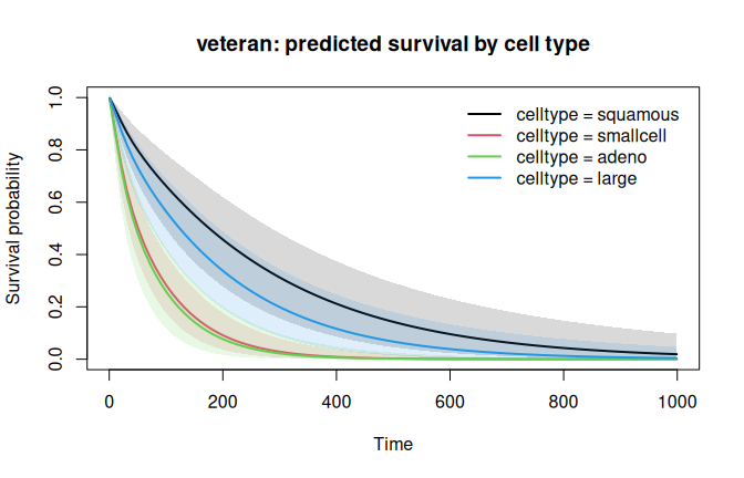
Factor covariates are given in newdata by their levels, as in
coxph():
fit_vet <- rpsurv(Surv(time, status) ~ trt + celltype, data = veteran, df = 3)
plot(fit_vet, newdata = data.frame(trt = 1, celltype = levels(veteran$celltype)),
     main = "veteran: predicted survival by cell type")
predict() also returns type = "hazard", "cumhaz", "link" (the
linear predictor), or "hr" (the instantaneous hazard ratio of
newdata versus newdata0, correct under time-varying effects), with
se.fit = TRUE adding delta-method 95% confidence limits for
"survival", "cumhaz", and "link". rmst_diff() gives the
difference in restricted mean survival time between two covariate
profiles, with a delta-method confidence interval:
rmst_diff(fit, newdata = data.frame(hormon = 1), newdata0 = data.frame(hormon = 0),
          tau = 2000, se.fit = TRUE)
#>        est       se    lower    upper
#> 1 161.5922 53.52856 56.67811 266.5062
Time-varying effects (non-proportional hazards)
A covariate’s value is fixed for a subject, but its coefficient can
be allowed to change over follow-up via its own spline in log time,
requested with tve:
fit_tve <- rpsurv(Surv(rectime, censrec) ~ hormon, data = brcancer,
                  df = 4, tve = "hormon", tve.df = 2)
coef(fit_tve)
#>     (Intercept)        s(logt)1        s(logt)2        s(logt)3        s(logt)4
#>    -19.19831045      2.93107392     -0.42391236      1.32596818     -0.87852652
#>          hormon hormon:s(logt)1 hormon:s(logt)2
#>     -2.34612306      0.32152113      0.03596688
A likelihood-ratio test of fit_tve against fit (both
maximum-likelihood fits, nested models) tests the proportional-hazards
assumption for hormon directly.
This is distinct from a time-varying covariate, where the
covariate’s value itself changes during follow-up. That is a
data-representation question, not a modeling one: split each subject’s
follow-up into intervals over which the covariate is constant and supply
counting-process data via Surv(start, stop, status). rpsurv detects
the 3-column Surv object and fits the left-truncated likelihood
automatically, correctly accounting for each interval’s dependence on
survival to its start time under the covariate value of the previous
interval. The same mechanism also handles ordinary left truncation
(delayed entry) when covariate values don’t change. See
vignette("rpsurv") for a full worked example and the underlying
likelihood.
Non-linear effects and effect curves
nle gives a numeric covariate a smooth non-linear effect g(x), a
restricted cubic spline in the covariate with nle.df degrees of
freedom (nle.df = 1 is the linear fit). It is specified separately
from tve, and a covariate may have both. tve.df and nle.df take a
single value or a vector named by covariate. Here age (x1) enters
non-linearly and hormon keeps its time-varying effect:
fit_nle <- rpsurv(Surv(rectime, censrec) ~ hormon + x1, data = brcancer,
                  df = 4, tve = "hormon", tve.df = 2, nle = "x1", nle.df = 3)
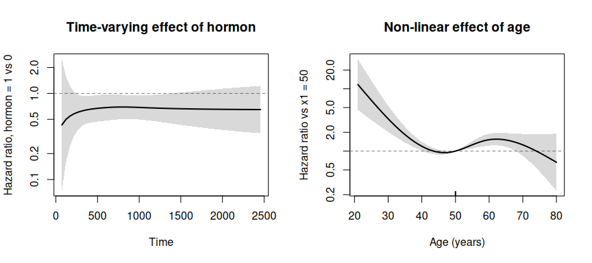
tvecurve() returns the time-varying effect (by default the log
instantaneous hazard ratio per unit increase, type = "hr"; or the
coefficient function beta(t), type = "link"), and nlecurve() returns
g(x) - g(ref). Both come with delta-method 95% confidence limits:
tvecurve(fit_nle, "hormon", times = c(500, 1000, 2000))
#>   time        est        se      lower       upper
#> 1  500 -0.3991813 0.1802581 -0.7524807 -0.04588199
#> 2 1000 -0.3747085 0.1652700 -0.6986316 -0.05078529
#> 3 2000 -0.4256658 0.2810353 -0.9764849  0.12515334

nlecurve(fit_nle, "x1", at = c(30, 40, 50, 60, 70), ref = 50)
#>    x       est        se       lower     upper
#> 1 30 1.1927967 0.2468867  0.70890769 1.6766858
#> 2 40 0.1781839 0.0840963  0.01335822 0.3430097
#> 3 50 0.0000000 0.0000000  0.00000000 0.0000000
#> 4 60 0.4218401 0.1117849  0.20274560 0.6409345
#> 5 70 0.2309416 0.2057613 -0.17234318 0.6342264
Their plot() methods draw the hazard ratio against time or against the
covariate, with its confidence band, a reference line at no effect and a
log y axis (add = TRUE overlays curves):
op <- par(mfrow = c(1, 2))
plot(tvecurve(fit_nle, "hormon"), main = "Time-varying effect of hormon")
plot(nlecurve(fit_nle, "x1", ref = 50), xlab = "Age (years)",
     main = "Non-linear effect of age")
par(op)
Diagnostics
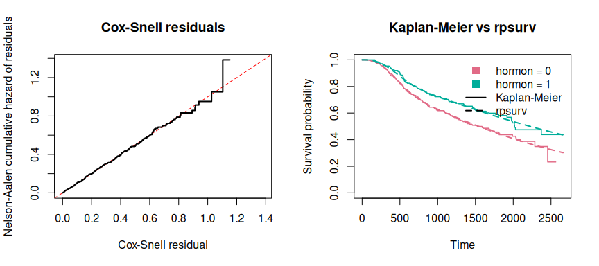
residuals() gives Cox-Snell, martingale or deviance residuals. The two
goodness-of-fit plots are also plot() types. type = "coxsnell" draws
the Nelson-Aalen cumulative hazard of the Cox-Snell residuals against
the residuals: a well-fitting model follows the diagonal. type = "km"
overlays the Kaplan-Meier estimate (solid) on the model’s average
predicted survival over the same subjects (dashed), overall or by group.
They are the same plots as coxsnell_plot() and km_compare_plot():
op <- par(mfrow = c(1, 2))
plot(fit, type = "coxsnell", main = "Cox-Snell residuals")
plot(fit, type = "km", by = "hormon", main = "Kaplan-Meier vs rpsurv")
par(op)
Validation
Coefficients, standard errors, and log-likelihoods agree with
rstpm2::stpm2 to 4-5 decimal places across all three scales (hazard,
odds, normal) and with flexsurv::flexsurvspline on the hazard
scale. See tests/testthat/test-rpsurv.R for the full parity suite,
which also covers left truncation, and
tests/testthat/test-components.R for the nle, tvecurve() and
nlecurve() checks.
Benchmark vs. rstpm2 and flexsurv
Wall-clock fit time (seconds, median of 3 runs) on simulated
Weibull-hazard data with two covariates, reproducible via
data-raw/benchmark.R (in the GitHub repository, not in the CRAN
tarball). flexsurv::flexsurvspline is much slower per fit, so it was
only run up to n = 20,000; rstpm2::stpm2 was run up to n = 200,000.
The speedup columns are the other package’s time divided by
rpsurv’s.
| n | rpsurv (s) | rstpm2 (s) | flexsurvspline (s) | speedup vs rstpm2 | speedup vs flexsurv |
|---|---|---|---|---|---|
| 1e+03 | 0.059 | 0.021 | 0.166 | 0.4 | 2.8 |
| 5e+03 | 0.055 | 0.075 | 0.618 | 1.4 | 11.2 |
| 2e+04 | 0.110 | 0.299 | 2.676 | 2.7 | 24.3 |
| 5e+04 | 0.144 | 1.200 | NA | 8.3 | NA |
| 1e+05 | 0.223 | 2.519 | NA | 11.3 | NA |
| 2e+05 | 0.440 | 5.954 | NA | 13.5 | NA |
| 5e+05 | 1.207 | NA | NA | NA | NA |
The same comparison with a time-varying effect (tve = "x1",
tve.df = 2; stpm2(..., tvc = list(x1 = 2))) and a non-linear effect
(nle = "x1", nle.df = 3; stpm2 with ns(x1) on the same knots, so
both fit the same model):
| model | n | rpsurv (s) | rstpm2 (s) | speedup vs rstpm2 |
|---|---|---|---|---|
| tve | 1e+03 | 0.033 | 0.019 | 0.6 |
| nle | 1e+03 | 0.032 | 0.028 | 0.9 |
| tve | 5e+03 | 0.061 | 0.085 | 1.4 |
| nle | 5e+03 | 0.059 | 0.095 | 1.6 |
| tve | 2e+04 | 0.106 | 0.333 | 3.1 |
| nle | 2e+04 | 0.103 | 0.375 | 3.6 |
| tve | 1e+05 | 0.247 | 3.619 | 14.7 |
| nle | 1e+05 | 0.231 | 3.601 | 15.6 |
rpsurv gets faster relative to the others as n grows: it does O(n)
work per optimizer step in one fused parallel pass over the
log-likelihood and its analytic gradient
(RcppParallel::parallelReduce), while the other two packages evaluate
the likelihood repeatedly at R level. Below a few thousand rows a fit
takes a few hundredths of a second in every package, and rstpm2 is
slightly faster there because of rpsurv’s fixed setup cost (spline
basis, starting values, reparameterisation). See vignette("rpsurv")
for the benchmark code.
Bundled datasets
rpsurv ships three datasets, each chosen for a specific feature of the
package rather than as a generic example:
brcancer: German breast cancer recurrence data (686 rows), the baseline fitting example used throughout this README and the vignette. Identical torstpm2::brcancer, bundled so examples do not requirerstpm2to be installed.veteran: Veterans’ Administration lung cancer trial (137 rows).celltypeis a well-known non-proportional-hazards effect, which makes this a direct illustration of thetveargument. Identical tosurvival::veteran.heart: Stanford heart transplant data (172 rows), already in counting-process (start,stop,event) format with a time-varyingtransplantcovariate. IllustratesSurv(start, stop, status)fitting on a real dataset rather than a constructed one. Identical tosurvival::heart.
Notes
scaleselects the transformation of the survival function the spline models:"hazard"(proportional hazards, the Royston-Parmar default),"odds"(proportional odds), or"normal"(probit).- Boundary knots default to the min/max of log time among events, and
interior knots to equally spaced centiles of log time among events,
matching
rstpm2/flexsurvconventions.nleknots are placed the same way on the covariate (range and equally spaced centiles). SystemRequirements: GNU make(forRcppParallel); no other external dependencies.