Datasets with Strong and Spurious Correlations

Provides datasets from Vigen (2015) rescued from the Internet Wayback Machine. These should be preserved for statistics introductory courses as these make it very clear that correlation is not causation.

Spurious correlations

The goal of spuriouscorrelations is to keep alive the amazing examples from Tyler Vigen. Unfortunately, as of 2023-10-09, the website is down as my students noticed. Therefore, I decided to use the snapshot from the Internet Wayback Machine to save the datasets from 2023-06-07.

Installation

You can install the CRAN version of spuriouscorrelations with:

install.packages("spuriouscorrelations")

You can install the development version of spuriouscorrelations with:

remotes::install_github("pachadotdev/spuriouscorrelations")

Example

The package covers multiple examples for different spurious (and curious) correlations.

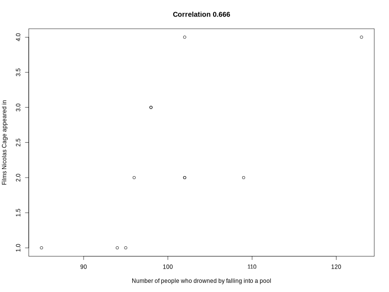
Here is a basic example which shows you how to plot a spurious correlation for the variables

• x: Number of people who drowned by falling into a pool
• y: Films Nicolas Cage appeared in

library(spuriouscorrelations)
library(tinyplot)

pool_drownings

#    year   x y
# 1  1999 109 2
# 2  2000 102 2
# 3  2001 102 2
# 4  2002  98 3
# 5  2003  85 1
# 6  2004  95 1
# 7  2005  96 2
# 8  2006  98 3
# 9  2007 123 4
# 10 2008  94 1
# 11 2009 102 4

cor(pool_drownings$x, pool_drownings$y)

# [1] 0.6660043

tinyplot(
  y ~ x,
  data = pool_drownings,
  main = sprintf("Correlation %s", round(cor(pool_drownings$x, pool_drownings$y), 3)),
  xlab = "Number of people who drowned by falling into a pool",
  ylab = "Films Nicolas Cage appeared in"
)

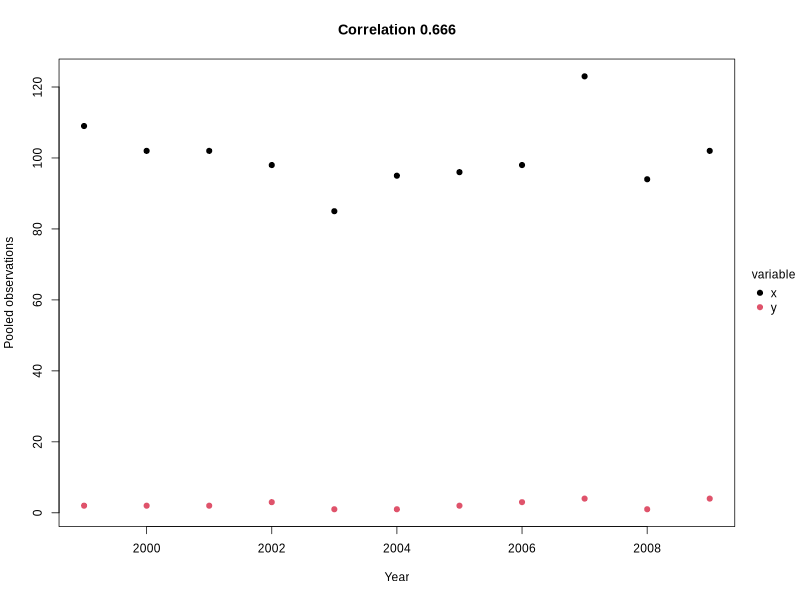
Converting the data to long format simplified plotting both variables per year:

pool_drownings_2 <- reshape(
  pool_drownings, 
  varying = c("x", "y"),  # columns to collapse
  v.names = "value",      # name of the new value column
  timevar = "variable",   # name of the new ID column
  times = c("x", "y"),    # values to populate the ID column
  direction = "long"      # target format
)

pool_drownings_2

#      year variable value id
# 1.x  1999        x   109  1
# 2.x  2000        x   102  2
# 3.x  2001        x   102  3
# 4.x  2002        x    98  4
# 5.x  2003        x    85  5
# 6.x  2004        x    95  6
# 7.x  2005        x    96  7
# 8.x  2006        x    98  8
# 9.x  2007        x   123  9
# 10.x 2008        x    94 10
# 11.x 2009        x   102 11
# 1.y  1999        y     2  1
# 2.y  2000        y     2  2
# 3.y  2001        y     2  3
# 4.y  2002        y     3  4
# 5.y  2003        y     1  5
# 6.y  2004        y     1  6
# 7.y  2005        y     2  7
# 8.y  2006        y     3  8
# 9.y  2007        y     4  9
# 10.y 2008        y     1 10
# 11.y 2009        y     4 11

tinyplot(
  value ~ year | variable, # "|" indicates the groping variable for the legend
  data = pool_drownings_2,
  main = sprintf("Correlation %s", round(cor(pool_drownings$x, pool_drownings$y), 3)),
  xlab = "Year",
  ylab = "Pooled observations",
  pch = 19 # solid dot shape
)

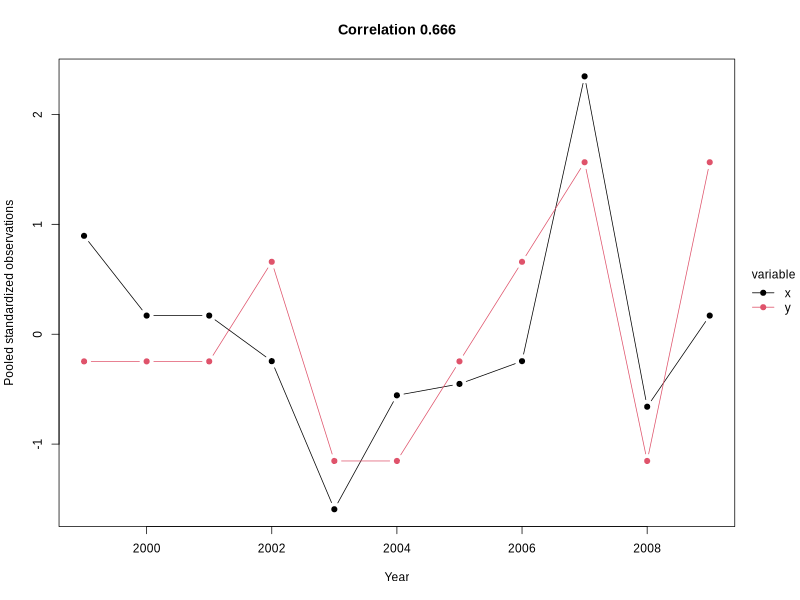
How about standarzing the variables to avoid the different scale visibility issue?

pool_drownings_3 <- pool_drownings

pool_drownings_3$x <- (pool_drownings_3$x - mean(pool_drownings_3$x)) / sd(pool_drownings_3$x)
pool_drownings_3$y <- (pool_drownings_3$y - mean(pool_drownings_3$y)) / sd(pool_drownings_3$y)

pool_drownings_3 <- reshape(
  pool_drownings_3, 
  varying = c("x", "y"),  # columns to collapse
  v.names = "value",      # name of the new value column
  timevar = "variable",   # name of the new ID column
  times = c("x", "y"),    # values to populate the ID column
  direction = "long"      # target format
)

pool_drownings_3

#      year variable      value id
# 1.x  1999        x  0.8952867  1
# 2.x  2000        x  0.1696333  2
# 3.x  2001        x  0.1696333  3
# 4.x  2002        x -0.2450258  4
# 5.x  2003        x -1.5926679  5
# 6.x  2004        x -0.5560201  6
# 7.x  2005        x -0.4523554  7
# 8.x  2006        x -0.2450258  8
# 9.x  2007        x  2.3465935  9
# 10.x 2008        x -0.6596849 10
# 11.x 2009        x  0.1696333 11
# 1.y  1999        y -0.2470999  1
# 2.y  2000        y -0.2470999  2
# 3.y  2001        y -0.2470999  3
# 4.y  2002        y  0.6589330  4
# 5.y  2003        y -1.1531327  5
# 6.y  2004        y -1.1531327  6
# 7.y  2005        y -0.2470999  7
# 8.y  2006        y  0.6589330  8
# 9.y  2007        y  1.5649658  9
# 10.y 2008        y -1.1531327 10
# 11.y 2009        y  1.5649658 11

tinyplot(
  value ~ year | variable, # "|" indicates the groping variable for the legend
  data = pool_drownings_3,
  main = sprintf("Correlation %s", round(cor(pool_drownings$x, pool_drownings$y), 3)),
  xlab = "Year",
  ylab = "Pooled standardized observations",
  pch = 19, # solid dot shape
  type = "b" # add line to see the trend clearly
)